Information Theory in Gambling Part I: Variance and the Kelly Criterion

04 Jul 2019

Let’s play a game. Imagine you have $100 and you’d like to maximize your money. You flip a weighted coin that comes up heads 60% of the time, and tails 40% of the time $x \sim \mathrm{Bernoulli}(p=0.6)$. You can play as many times as you would like. How much would you bet?

The most intuitive answer may not be the optimal one. Well let’s look at the two extremes. If you choose to bet $0, i.e. not play the game at all, you will leave with $100 with probability 1. If you bet the entire $100, you have a 60% of doubling up, and 40% of leaving with nothing. That gives you an expected value (EV) of 0.6(200) + 0.4(0) = 120. Since $120/$100 = 1.2, in the long run you would expect to make 1.2x your bet. So you might naturally think that the optimal strategy is to always bet all your money. But what if it lands on tails the first time? Then you can no longer continue to play the game since you will have no more money. In poker language, you won’t be able to realize your equity because even though in the limit of infinite wealth, you will make money, you can’t withstand the variance of any individual flip. In fact, in the limit of infinite games, you will go broke with probability 1. So it seems like the optimal betting strategy is somewhere in between the two, and should probably vary according to the size of your budget.

Kelly Criterion

This problem was studied by mathmetician John Kelly in 1956 while he was an associate under Claude Shannon at Bell Labs. Kelly proposed maximizing the expected (log) wealth [1]. For a binary game that offers $l$ odds (you receive $l$ times your bet if you win not including your bet) on an outcome with probability $q$, this would be: \begin{equation} \mathbb{E}[R] = q \log(1 + xl) + (1 - q)\log (1-x) \end{equation}

where $x$ is the proportion of your wealth to bet. To find $x$ which maximizes this expression, we simply take the derivative and set it equal to zero: \begin{align} \frac{d\mathbb{E}[R]}{dx} &= q\frac{d}{dx} \log(1 + xl) + (1-q)\frac{d}{dx}\log(1-x) \newline &=\frac{ql}{1+xl} - \frac{1-q}{1-x}= 0 \end{align}

Rearranging to solve for $x$: \begin{equation} x = q - \frac{1 - q}{l} \end{equation}

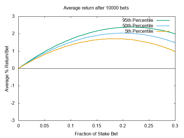
This is commonly referred to as the Kelly bet. For our game above, plugging 0.6 for $q$ and 1 for $l$, we get 0.6-0.4 = 0.2. If we plot our wealth as a function of our bet, we see that the optimal bet size is indeed 20% of our wealth.

returns

In limit of infinite games, the Kelly bet will yield the highest payoff than any other bet. This formula (and its variants) is widely used in Blackjack, sports betting, and financial investing to great success [4].

Information Theoretic Approach

Unsurprisingly, Kelly studied this problem from the perspective of information theory and posed the question as follows: suppose you were able to communicate by phone with your future self. Naturally, being the ambitious gambler you are, you use this opportunity to get the results of events that haven’t occurred yet - making that perfect March Madness bracket, investing in bitcoin, etc. However, your telegram is noisy - it only transmits the correct signal probabilistically. How confident can you be in your bet?

If you bet a fraction $x$ of your wealth, then your wealth $R$ at round $N$ is: \begin{equation} R_N = (1+x)^W(1-x)^LV_0 \end{equation} where $W$ and $L$ are the number of correct and incorrect bets respectively. So as before, we want to maximize the expected wealth (which is also the maximum rate of growth) over an infinite number of games: \begin{align} \mathbb{E}[R] &= \lim_{N\to\infty}\bigg[\frac{W}{N}\log(1+x) + \frac{L}{N}\log(1-x)\bigg] \newline &= q \log (1+x) + (1-q) \log(1-x) \end{align} $q$ is the probablity receiving the correct message which makes this the same expression as the one we derived in the previous section. So another way to think about it is, assuming you bet correctly, the maximum exponential rate of growth of your capital is equal to the rate of transmission of information over your telegram.

Multiple Outcome Games

The Kelly Criterion generalizes similarly to games with a multiple outcomes (e.g. horse racing). Given a game with $s, r \in S$ outcomes, \begin{equation} \mathbb{E}[R] = \sum_{s,r} p(s, r) \log a(s|r) + \sum_s p(s) \log\alpha_s \end{equation} where $p(s)$ is the probability that message $s$ was sent by your future self, $a(s|r)$ is the probability you bet on $s$ after receiving a message that tells you to bet on $r$ and $\alpha_s$ is the odds paid for event $s$ plus your original bet (derivation can be found in [1]). We can set $\sum_s a(s|r) = 1$ since we can place bets that cancel out according to $\alpha_s$. We can maximize the above expression by setting $a = q$ since \begin{align} a(s|r) &= \frac{p(s, r)}{\sum_k p(k, r)} \newline &= \frac{p(s,r)}{q(r)} \newline &= q(s|r) \end{align} This says that the optimal betting strategy is to bet according to $q(s|r)$ only, so your best bet is actually to ignore the posted odds!

If we recognize both terms in the expected wealth equation as entropy terms of our communication channel, we can derive capital as a function of the transmission rate: \begin{align} \mathbb{E}[R] &= \sum_s p(s) \log\alpha_s + \sum_{s,r} p(s, r) \log q(s|r) \newline &=H(\alpha) - H(X|Y) \end{align} which is the channel transmission rate [3].

Some Takeaways

So… that’s it right? If you bet according to this formula, you should never go broke …right? Well, maybe. In Part II, we’ll see if we can design a game that will bankrupt a seemingly optimal player. But before you book your one way trip to Las Vegas, remember that the Kelly criterion makes some crucial assumptions:

You can play the game an infinite amount of times. In a game where you only have a limited number of rounds, the Kelly bet is not optimal
You are betting your entire lifeline. If you can replenish your bankroll, (e.g. in a cash poker game), the most profitable strategy is to bet all your wealth.
You can compute your probability of winning exactly. In practice (stock markets, etc), this is very difficult or impossible, so you’re often recommended to bet less than the Kelly bet.
The formula does not address variance, since it only computes an expectation: in practice, you may deviate (arbitrarily far) from the expected profit.

The exact coin flip game described in the first section was actually conducted in a research study [2] and perhaps unsurprisingly, most participants played far from optimal. 28% of the participants busted out, and 21% reached the maximum payout of 10x their bankroll. 67% bet tails (the less likely outcome) at some point during the experiment. The reasons for these biases have been thoroughly explored in cognitive science, psychology, and economics, which I’ll get to in Part 2. But the next time you find yourself in a casino, you’ll know how to bet to take down the house. Or at the very least you won’t end up like this guy:

lechiffre

References

[1] Kelly, J. L. A New Interpretation of Information Rate. 1965.
[2] Haghani & Dewey. Rational Decision-Making under Uncertainty: Observed Betting Patterns on a Biased Coin.. 2016.
[3] Shannon, C. E. A Mathematical Theory of Communication.. 1948.
[4] Thorp E. The Kelly Criterion in Blackjack Sports Betting, and the Stock Market. 2006.